The
SAM file format and its specification
is pretty amazing, but also terse and abstract. To really understand what is
going on with your reads, you need to play with real-world data and learn from
tutorials.
I’ll relay some things I’ve learned over the years, focused on how SAM
concepts relate to structural variants.
Disclaimer: I’m a developer of JBrowse 2. This document has some screenshots and links for it, feel free to try it at https://jbrowse.org.
Basics
What is a SAM file, and how does it relate to BAM and CRAM?
-
A
SAMfile generally contains “reads” from a sequencer, with information about how they are mapped to a reference genome 12. -
It is generally produced when an aligner takes in raw, unaligned reads (often stored in
FASTQformat files) and aligns them to a reference genome 3. -
A
SAMfile is a text format that you can read with your text editor.BAMandCRAMare compressed representations of theSAMformat.
You generally see BAM or CRAM in the wild instead of SAM since the files
are very large, so the compressed versions are better to store on disk.
See Appendix E on how to convert between SAM/BAM/CRAM.
What is in a SAM/BAM/CRAM file?
A SAM file contains a “header” and a series of “records”.
What is a SAM “record”?
A record is a single line in a SAM file, and it generally corresponds to a
single read, but as we will see, a split alignment may produce multiple records
that refer to the same source read.
Note that the words “read” and “record” are sometimes used interchangeably, but
record has the more specific meaning of being a single line in the SAM file.
What are tags in a SAM file?
A SAM file has a core set of required fields, and then an arbitrary list of
extra columns called tags. The tags have a two-character abbreviation like MQ
(mapping quality) or many others. They can be upper or lower case. Upper case
tags are reserved for official usages (except those starting with X, Y, or Z,
which are reserved for local/user-defined use). See
SAMtags.pdf for more
details.
What is a CIGAR string, and how do you interpret it?
A CIGAR string is a “compact idiosyncratic gapped alignment report”. It tells
you about insertions, deletions, and clipping. It is a series of “operators”
with lengths.
Insertion example:
50M50I50M
That would be 50bp of matching bases (50M), followed by a 50bp insertion
(50I), followed by another 50bp of matches (50M). The 50bp insertion means
the read contains 50 bases in the middle, which did not match the reference
genome that you are comparing the read to.
Clipping example:
50S50M50S
This means that 50bp matched (50M in the middle of the CIGAR string) and
both sides of the read are soft-clipped. The clipping means the aligner was not
able to align the reads on either side.
Notes:
-
Finding mismatches: A
CIGARstring match like50Mmeans 50 bases “matched” the reference genome, but that only means that there are no insertions or deletions in those 50 bases. There could be underlying mismatches in the read compared to the reference. Note: there is also “extendedCIGAR” that replacesMwith=(exact match) andX(mismatch). Also see Appendix D on theMDtag and finding where the mismatches are, but note thatMDtag is tricky -
Ambiguity of representation: A
CIGARstring with insertions and deletions could be50M1D1I50M. This string had a 1bp deletion and a 1bp insertion back-to-back. This could be just a mismatch! There is ambiguity in sequence alignment representations. Downstream programs must accommodate this. -
Split records and soft-clipping: A
CIGARstring with soft-clipping500S50Mthis means that 500 bases of the read were not aligned at this position, but 50 bases were!
See SAMv1.pdf for all the CIGAR operators.
If you are working with SAM data, you will often write loops that directly
parse CIGAR strings. See Appendix B for handy functions for parsing CIGAR
strings. Don’t fear the CIGAR!
Note regarding soft clipping: this will be discussed further in this post, but “supplementary alignments” might indicate that e.g. those 500 bases that were soft-clipped aligned to another region on the genome.
How do you determine “start” and “end” and “strand” of a record?
SAM records do not have easy-to-interpret “start” and “end” and “strand” fields
like, say, lines in a BED file do
Instead, each SAM record has:
- A single
POScoordinate - A
CIGARstring - A flags field, that might say “read reverse complemented”
Using this, you can find the “end” coordinate of a record by starting at the POS
coordinate and enumerating the reference-consuming operators of the CIGAR:
matches (M/=/X), deletions (D), and skips (N). Processing the whole CIGAR
effectively gives you the “end” coordinate on the reference genome, so “end” is
derived from the CIGAR. The “start” field corresponds to the POS field
What are “forward” and “reverse” strand reads?
Reads can align to the “forward strand” of the reference genome (e.g. it matches the DNA letters as written in the reference genome FASTA file), resulting in “forward strand reads”.
Or, they can align to the reverse complement of the DNA in the reference genome, resulting in “reverse strand reads”.
Strandedness is recorded for each record in the SAM/BAM/CRAM file by having the SAM flags bitwise flag 16 enabled (https://broadinstitute.github.io/picard/explain-flags.html), where this flag is called “read reverse strand”.
Do you count backwards with the CIGAR for reverse strand reads?
As mentioned above, you get the “start” and “end” by processing the CIGAR, so
one might wonder whether you count “downwards” from POS for reverse strand
reads. This is actually not correct though
Here is what the SAM spec has to say about this
“
POSis the 1-based leftmost mapping POSition of the firstCIGARoperation that “consumes” a reference base”
And regarding CIGAR and other fields:
“For segments that have been mapped to the reverse strand, the recorded
SEQis reverse complemented from the original unmapped sequence andCIGAR,QUAL, and strand-sensitive optional fields are reversed and thus recorded consistently with the sequence bases as represented”
That is a little bit of a mind boggle but effectively, no matter whether the
record is forward or reverse strand, you count upwards when processing the
CIGAR.
You can see in an example of this in SAMv1 section 1.1 — the read r001/2 is a
“reverse strand” read, and its POS, or “start” position, is 37, and then the
CIGAR (9M, 9 matches) counts upwards from there, giving it an “end” position
of 45.
How are reads ordered in a SAM file?
When you run an aligner program like bwa or minimap2, you type e.g.
minimap2 -a reference_genome.fa reads.fq > out.sam
out.sam will be ordered in the same order as the fastq. For preparation for
loading into analysis tools or genome browsers, we will often sort the reads
using samtools sort which will group by chromosome name, and then increasing
in coordinate start position. Then samtools index creates an index file (e.g.
bam.bai, cram.crai). The index file lets you quickly query the reads in a
specific genomic region (e.g. with samtools view myfile chr10:1000-2000). See
Appendix G for how this indexing actually works.
What happens to reads that don’t align to the genome?
If a read failed to align to the reference genome, it may still be in your SAM
file, marked as unmapped using the flag column. Sometimes, “dumpster diving”
(looking at the unmapped records from a SAM file) can be used to aid
structural variant searches (e.g. there may be novel sequence in there not from
the reference genome that could be assembled)
Detecting SVs from long reads
Long reads offer a wide array of methods for detecting SVs
- Small insertions/deletions: Long reads can completely span moderate sized
insertions and deletions, indicated by
IorDin aCIGARstring. - Large insertions/deletions: If a long read does not completely span an insertion or deletion, it may be split aligned on either side of the SV or could be soft/hard clipped where it can’t align all the way through an insertion.
- Translocations: A split long alignment can span long-range or even inter-chromosomal translocations, so part of the read maps to one chromosome and one part maps to the other
- Inversions: A split alignment can span an inversion. In this case, long reads can be split into multiple parts, one part of it aligns in the reverse orientation, while the other part aligns in the forward orientation
There are many other methods for detecting SVs from long reads — not all use mapped reads (some use de novo assembly for example) — but mapped-read methods are still useful to know.
What are split/supplementary/chimeric alignments?
Split alignments, or chimeric alignments, are alignments where part of the read
maps to one place, and another part to another. For example, part of a long read
may map to chr1 and part of it maps to chr4. It is worth reading the
definition of “Chimeric alignment” from
SAMv1.pdf when you get the
chance.
As SAMv1.pdf tells us, one
record is marked as “representative”, sometimes also called the “primary”
record, while the other components of the split read are marked “supplementary”,
given the 2048 flag. The “primary” record generally has a SEQ field that
represents the entirety of the original read’s sequence (with CIGAR soft
clipping operators saying which part of that sequence aligned), and the
“supplementary alignments” will have SEQ field but sometimes just segments of
the original read’s sequence with CIGAR hard clipping operators indicating that
it is partial.
Supplementary alignments are especially common with long reads and can signal structural variants: a read may split across a chromosomal fusion, align to either side of a large deletion, or span an inversion (part aligning forward, part reverse).
There is no limitation on how many splits might occur so the split can align to
3, 4, or more different places. Each part of the split puts a new line in the
SAM file, and note that all the records also have the same read name, or QNAME
(first column of SAM).
What are secondary alignments/multi-mappers?
Secondary alignments generally come from “multi-mappers” where the entire read
maps equally well (or at least somewhat equally well) to, say, somewhere on both
chr4 and chr1. “Multi mapping” results in secondary alignments, while split
reads result in supplementary alignments. See “Multiple mapping” in the
SAMv1.pdf for the definition
of multi-mapping. Note also that secondary alignments sometimes are missing the
SEQ field entirely too, see
https://github.com/lh3/minimap2/issues/458#issuecomment-516661855.
I wrote a tool called secondary_rewriter to add the SEQ field back to
secondary alignments, which may help in some cases.
What is the SA tag?
The SA tag is outputted on each part of the supplementary/split/chimeric
alignment, e.g. the primary contains an SA tag that refers to information
(e.g. the location) of where all the supplementary alignments were placed, and
each of the supplementary alignments also contains an SA tag that refers to
the primary alignment and each other supplementary alignment.
Fun fact: The SA tag conceptually can result in a ‘quadratic explosion’ of
data, because each part of the split contains references to every other part.
For example, if a read is split into 4 pieces, then each record would have an
SA tag with 3 segments, so 3*4 segments will be documented in the SA tag.
In many cases, this is not a problem, but if you imagine a finished chromosome
aligned to a draft assembly, it may get split so many times that this could be a
factor.
See SAMtags.pdf for more
info on the SA tag.
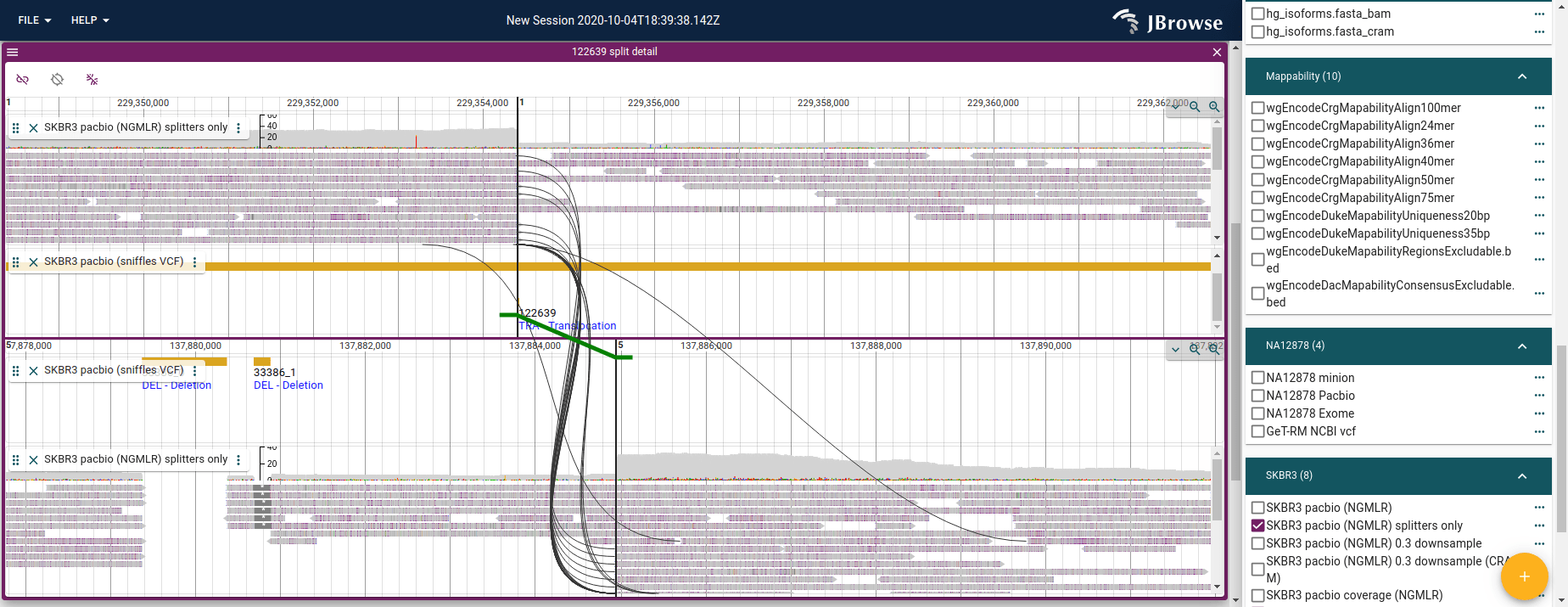
Visualizing split reads across a breakend or translocation
For an inter-chromosomal translocation, JBrowse 2’s “breakpoint split view” visualizes support for the event, showing reads that are split-aligned across the SV (and connections between paired-end reads across it too).
The SV inspector
workflow helps you set these up, and you can launch the breakpoint split view
from it. Both work best on Breakends (VCF 4.3 section 5.4) and <TRA> events
from VCF, or BEDPE SV calls.
Visualizing a ‘read vs reference’ view given a split alignment
Given any one record of a split read, we can reconstruct what the whole read
looks like compared to the reference genome. We don’t need the primary
specifically: the record’s SA tag lists every other piece, so the record plus
its SA tag describe the whole read.
The primary is special in one respect: it carries the SEQ of the entire read,
so it’s where the full read sequence lives if you want to display the bases.
(Whether supplementary records also carry the full SEQ depends on the aligner:
minimap2 and bwa hard-clip them by default so they store only their aligned
portion, but -Y makes them soft-clip and keep the entire SEQ.) JBrowse 2
implements this reconstruction with a synteny-style rendering. [1]
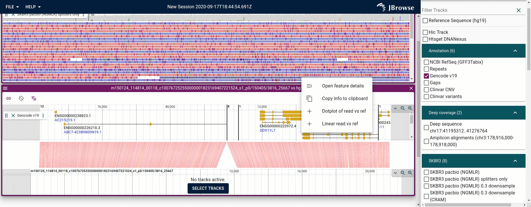
Figure showing JBrowse 2 piecing together a long read vs the reference genome from a single read
To do this, JBrowse takes the CIGAR of the record you started from plus each
piece in its SA tag, and sorts them by the length of the clip at the start of
the read, counting soft (S) and hard (H) clips alike (since supplementary
records may be either, depending on the aligner). A larger leading clip means
the piece starts further along the read, so the clip lengths give the order of
the pieces — telling us where each came from in the original read, which we plot
in a synteny-style display.
[1] Similar functionality also exists in GenomeRibbon https://genomeribbon.org
SAM vs VCF - Breakends vs split alignments
A nice property of SAM is that from a single record I can reconstruct the
“derived” genome around a region of interest. The SA tag is just a set of
linear alignments that piece together easily, and you only need that one record
to do it.
Doing the same from the VCF Breakend specification (section 5.4 of
VCF4.3.pdf) is harder: a
Breakend is only an edge in a graph (sequences are the nodes), so reconstructing
a structural variant means building that graph and decoding paths through it. An
inversion, for example, may take 4 VCF records to express. Some tools do
tackle this — the GRIDSS / PURPLE / LINX pipeline reconstructs derivative
chromosomes from breakends, and so does my
derivative-chromosome-utils
— but it remains more involved than piecing together an SA tag.
The catch with single reads is that they can be noisy (contain errors). de
novo assembled contigs can also be stored in SAM format and are much less
noisy, being built from many reads.
Haplotype-tagged reads
A new trend has been to create SAM/BAM/CRAM files with tagged reads, which
tells us which haplotype a read was inferred to have come from. This is commonly
done with the HP tag, which might have HP=1 and HP=2 for a diploid genome.
Tools like whatshap can add these tags to a SAM file, and IGV and JBrowse 2
can color and sort by these tags.
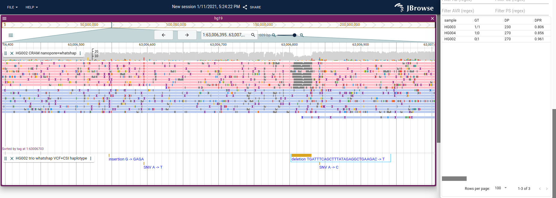
Screenshot of JBrowse 2 with the “Color by tag” and “Sort by tag” settings
enabled (coloring and sorting by the HP tag), letting us see that only one
haplotype has a deletion. Tutorial for how to do this in JBrowse 2 here:
https://jbrowse.org/jb2/docs/user_guides/alignments_track/#sort-color-and-filter-by-tag
How do you detect SVs with paired-end reads?
Distance between pairs being abnormally large or short
The distance between pairs is encoded by the TLEN column. For well-mapped
pairs it is relatively constant, called the “insert size”, and comes from how
paired-end sequencing reads both ends of a fragment.
But, if you are mapping reads vs the reference genome, and you observe that they are abnormally far apart, say 50kb apart instead of 1kb apart, this may indicate that your sample contains a deletion relative to the reference.
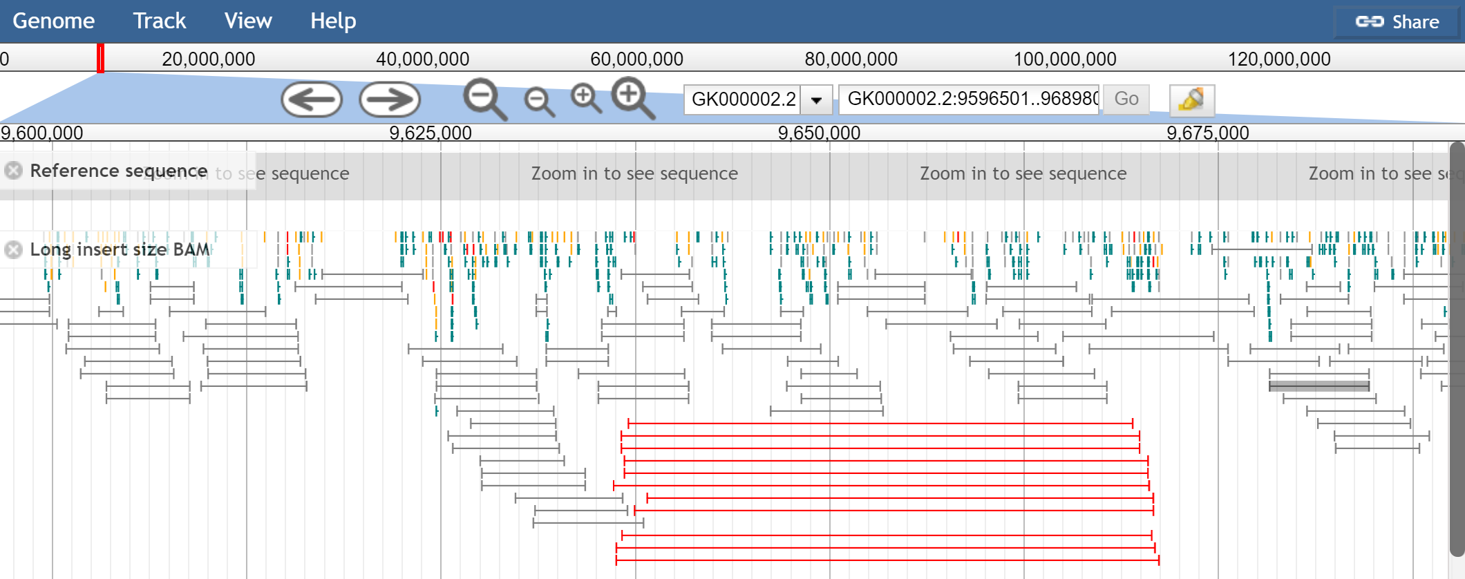
Screenshot of JBrowse 1 with “View as pairs” enabled with “mate paired” sequencing, and large insert size colored as red (from https://jbrowse.org/docs/paired_reads.html). Note that some of JBrowse 1’s View as pairs features are not yet available in JBrowse 2
Mate pairs vs paired end reads
“Mate paired” reads have a larger distance between pairs (aka the insert size is larger). Think: mate pairs have 2-5kb between pairs instead of a couple hundred bp. Mate pairs can be useful in scaffolding de novo genome assemblies since the larger range can span gaps, giving evidence that multiple contigs are connected.
“Paired-end” reads typically have like 200-500bp distance between pairs (aka, the insert size).
The above JBrowse screenshot shows mate pairs. Note that mate pairs have a different pair orientation, and pairs don’t necessarily point at each other, they “point away from each other” in normal conditions due to how the library is constructed. See Appendix A for more info.
Linked reads aka simulated long reads
Briefly: linked reads are another method that uses short reads but gives long read information, by tagging short reads that came from the same long molecule with a shared barcode. Note that 10x Genomics, the company that originally popularized this method, has since discontinued commercial linked-read sequencing to focus on single cell. https://www.10xgenomics.com/products/linked-reads
An abundance of reads being “clipped” at a particular position
This can indicate that part of the reads map well, but then there was an abrupt stop to the mapping. This might mean that there is a sequence that was an insertion at that position, or a deletion, or a translocation.
The clipping is indicated by the CIGAR string, either at the start or end of
it by an S or an H. The S indicates “soft clipping”, and indicates that
the sequence of the clipped portion can be found in the SEQ field of the
primary alignment. The H is hard clipped, and the sequence that is hard
clipped will not appear in the SEQ.
Screenshot of JBrowse 2 showing blue clipping indicator with a “pileup” of soft-clipping at a particular position shown in blue. The clipping is an “interbase” operation (it occurs between base pair coordinates) so it is plotted separately from the normal coverage histogram.
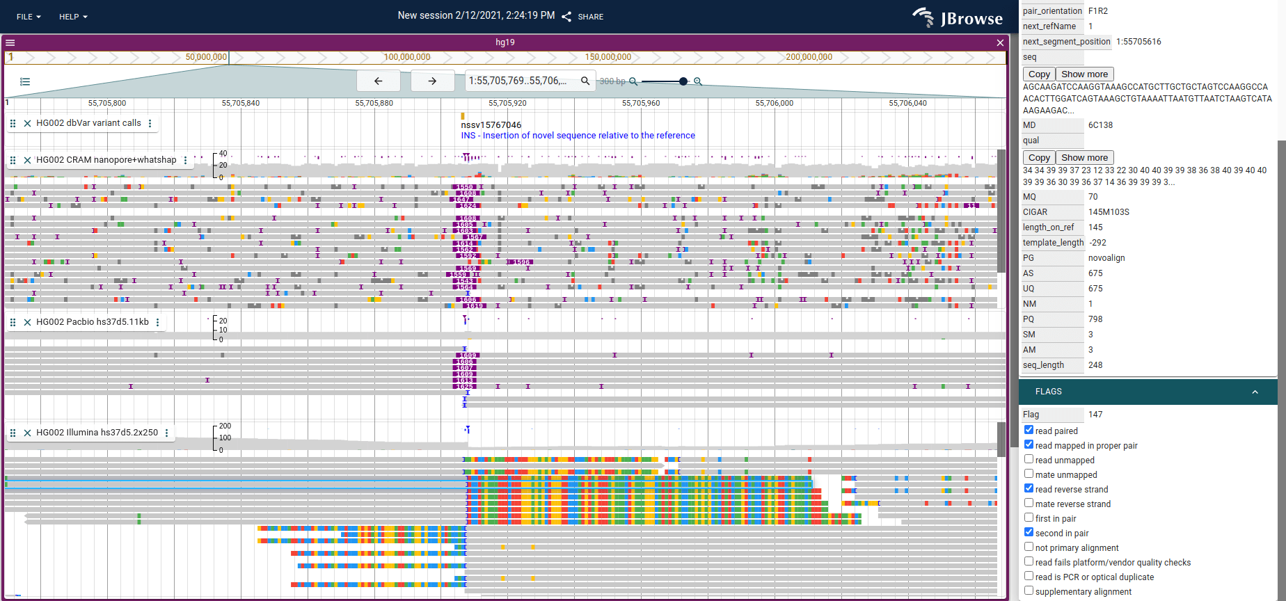
Screenshot of JBrowse 2 showing an insertion with Nanopore (top), PacBio
(middle) and Illumina short reads. The long reads may completely span the
insertion, so the CIGAR string on those have an I operator and are indicated
by the purple triangle above the reads. For the short reads, the reads near the
insertion will be clipped since they will not properly map to the reference
genome and cannot span the insertion. The “Show soft clipping” setting in
JBrowse 2 and IGV can be used to show visually the bases that extend into the
insertion (shown on the bottom track).
Unexpected pair orientation
With standard paired end sequencing, the pairs normally point at each other
forward          reverse
--->             <---
If the stranded-ness of the pair is off, then it could indicate a structural variant. See Appendix A for a handy function for calculating pair orientation.
This guide from IGV is helpful for interpreting the pair directionality with patterns of SVs using “Color by pair orientation”
https://software.broadinstitute.org/software/igv/interpreting_pair_orientations
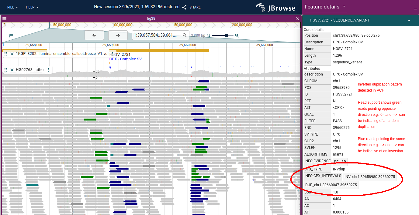
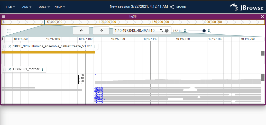
Figure: JBrowse 2 showing an inverted (tandem) duplication in 1000 genomes data.
It uses the same coloring as IGV for pair orientation. The tandem duplication
can produce green arrows which have reads pointing in opposite directions e.g.
<-- and -->, while blue arrows which can indicate an inversion point in the
same direction e.g. --> and -->
Caveat about TLEN
Note that TLEN is a field in the SAM format that is somewhat ill-defined, at
least in the sense that different tools may use it differently
https://github.com/pysam-developers/pysam/issues/667#issuecomment-381521767
If needed, you can compute the distance yourself from the paired records, but I
haven’t had trouble relying on the TLEN in the data files.
Calling copy number variants with your short or long reads
Another type of SV you can get from SAM files is copy number variants (CNVs).
Looking at depth-of-coverage for abnormalities can reveal them; a tool like
mosdepth quickly produces a file of coverage across the genome.
Be aware that if you are comparing the coverage counts from different tools,
they have different defaults that may affect comparison. Some discard QC_FAIL,
DUP, and SECONDARY flagged reads. This is probably appropriate, and
corresponds to what most genome browsers will display (see
https://gist.github.com/cmdcolin/9f677eca28448d8a7c5d6e9917fc56af for a short
summary of depth calculated from different tools)
Both long and short reads can be used for CNV detection; long reads may be more accurate thanks to better mapping through difficult regions.
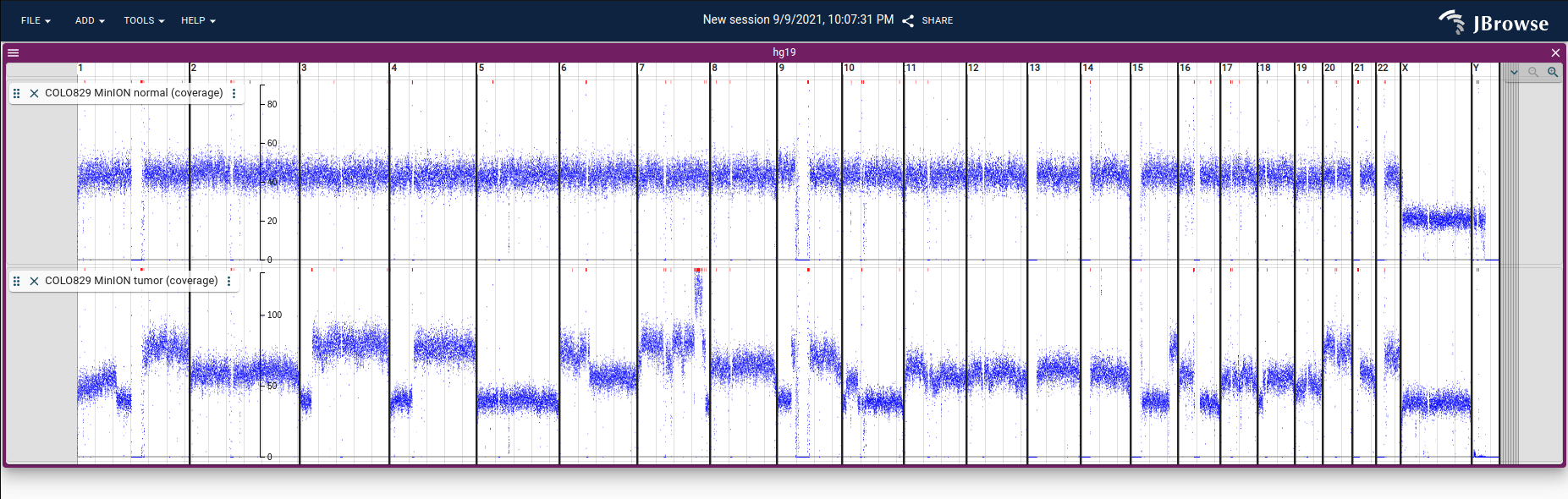
Screenshot showing coverage in BigWig format from nanopore reads on normal and
tumor tissue from a melanoma cancer cell line (COLO829) plotted using JBrowse 2.
This coverage data is calculated from nanopore sequencing from
here using
mosdepth, converted from BedGraph to
BigWig, and loaded into JBrowse 2. See
(demo
and
tutorial)
The future, with graph genomes and de novo assemblies
Currently, SV visualization is mostly based on comparing data to a reference
genome (and SAM is a signature of this: it stores everything in reference
coordinates). In the future it may look more like comparative genomics,
comparing an SV to a population-specific or graph-genome reference.
de novo assembly has more power to detect SVs than some read-based methods (https://twitter.com/lh3lh3/status/1362921612690010118/photo/1), so as assembled genomes improve and become more widespread, we may see a shift in how SVs are called. I’d also like to see fast ‘on the fly’ gene prediction on assembled genomes, to see what SNPs or altered splicing look like in duplicated gene copies.
Fun fact: the
GAF
(graphical alignment format) is a strict superset of
PAF (pairwise alignment
format) by storing graph node labels in the target name slot of PAF, and can
refer to an rGFA (reference genome graph)! Looking forward to the graph genome
world.
Conclusion
Algorithms that call structural variants face many challenges, but understanding how the reads are encoded in SAM format, and seeing what they look like in the genome browser is a useful first step to gaining a better understanding.
In summary, some of the signatures of SVs may include:
- Aberrant insert size (
TLEN) detection (longer for deletion, shorter for insertion) - Aberrant pair orientation (pairs are not pointing at each other)
- Split-read detection (
SAtag) CIGARstring processing (Doperator for deletions,Ioperator for insertions)- Over-abundance of clipping (
SorHoperators inCIGAR) - Depth of coverage changes for CNVs
- Aligning de novo assembly vs a reference genome (https://twitter.com/lh3lh3/status/1362921612690010118/photo/1)
That last point is worth expanding on: aligning a de novo assembly to a
reference can output SAM, but it can also output
PAF format, which can be
loaded into the JBrowse 2 synteny views. The techniques for detecting SVs from
PAF are fundamentally similar to those listed above, but may look a bit
different (see the cs tag in PAF for example, which is a modified
CIGAR-like string).
If you have any ideas I should include here, let me know!
Appendix A: Interpreting pair orientation
This is fairly low-level, but it’s a handy utility for determining pair orientation from a single SAM/BAM/CRAM record.
// @param flags - flags from a single read
// @param ref - this read's RNAME (reference sequence name)
// @param rnext - the RNEXT field, used to check the mate is on the same reference
// @param tlen - the TLEN field from SAM
// @return e.g. F1R2 normal paired end orientation
function getPairOrientation (
flags : number ,
ref : string ,
rnext : string ,
tlen : number ,
) {
// this read is not unmapped &&
// this read's mate is also not unmapped &&
// this read's mate is on the same reference genome (RNEXT '=' means same as RNAME)
if ( ! ( flags & 4 ) && ! ( flags & 8 ) && ( rnext === '=' || ref === rnext )) {
const s1 = flags & 16 ? 'R' : 'F'
const s2 = flags & 32 ? 'R' : 'F'
let o1 = ' '
let o2 = ' '
// if first in pair
if ( flags & 64 ) {
o1 = '1'
o2 = '2'
}
// else if second in pair
else if ( flags & 128 ) {
o1 = '2'
o2 = '1'
}
const tmp = []
if ( tlen > 0 ) {
tmp [ 0 ] = s1
tmp [ 1 ] = o1
tmp [ 2 ] = s2
tmp [ 3 ] = o2
} else {
tmp [ 2 ] = s1
tmp [ 3 ] = o1
tmp [ 0 ] = s2
tmp [ 1 ] = o2
}
return tmp . join ( '' )
}
return null
}
Then this can be broken down further by orientation type
- Paired end reads are “fr”
- Mate pair reads are “rf”
So you can interpret e.g. F1R2 in relation to being a paired end read (fr) or mate pair (rf) below and with this link https://software.broadinstitute.org/software/igv/interpreting_pair_orientations
{
"fr" : {
"F1R2" : "LR" ,
"F2R1" : "LR" ,
"F1F2" : "LL" ,
"F2F1" : "LL" ,
"R1R2" : "RR" ,
"R2R1" : "RR" ,
"R1F2" : "RL" ,
"R2F1" : "RL"
},
"rf" : {
"R1F2" : "LR" ,
"R2F1" : "LR" ,
"R1R2" : "LL" ,
"R2R1" : "LL" ,
"F1F2" : "RR" ,
"F2F1" : "RR" ,
"F1R2" : "RL" ,
"F2R1" : "RL"
}
}
Appendix B - CIGAR parsing
// @param cigar: CIGAR string in text form
// @returns an array of elements like ['30','M', '2','I', '50','M', '40','D']
// which you can consume in a loop two elements at a time
function parseCigar ( cigar : string ) {
return cigar . split ( / ([MIDNSHPX=]) / )
}
Then parse the returned array two at a time
// this function does nothing, but is informative for how to interpret a
// CIGAR string
// @param cigar - CIGAR string from record
// @param readSeq - the SEQ from record
// @param refSeq - the reference sequence underlying the read
function interpretCigar ( cigar : string , readSeq : string , refSeq : string ) {
const opts = parseCigar ( cigar )
let qpos = 0 // query position, position on the read
let tpos = 0 // target position, position on the reference sequence
// opts will be an array like this ['30','M', '2','I', '50','M', '40','D']
// which we parse two elements at a time
for ( let i = 0 ; i < opts . length ; i += 2 ) {
const len = + opts [ i ]
const op = opts [ i + 1 ]
// do things. refer to the CIGAR chart in SAMv1.pdf for which operators
// "consume reference" to see whether to increment
if ( op === 'M' || op === '=' ) {
// matches consume query and reference
const refMatch = refSeq . slice ( tpos , tpos + len )
const readMatch = readSeq . slice ( qpos , qpos + len )
for ( let i = 0 ; i < len ; i ++ ) {
if ( refMatch [ i ] !== readMatch [ i ]) {
// SNP at this position
}
}
qpos += len
tpos += len
}
if ( op === 'I' ) {
// insertions only consume query
// sequence of the insertion from the read is
const insSeq = readSeq . slice ( qpos , qpos + len )
qpos += len
}
if ( op === 'D' ) {
// deletions only consume reference
// sequence of the deletion from the reference is
const delSeq = refSeq . slice ( tpos , tpos + len )
tpos += len
}
if ( op === 'N' ) {
// skips only consume reference
// skips are similar to deletions but are related to spliced alignments
tpos += len
}
if ( op === 'X' ) {
// mismatch using the extended CIGAR format
// could lookup the mismatch letter in a string containing the reference
const mismatch = refSeq . slice ( tpos , tpos + len )
qpos += len
tpos += len
}
if ( op === 'H' ) {
// does not consume query or reference
// hardclip is just an indicator
}
if ( op === 'S' ) {
// softclip consumes query
// below gets the entire soft clipped portion
const softClipStr = readSeq . slice ( qpos , qpos + len )
qpos += len
}
}
}
Note for example, that to determine how long a record is on the reference sequence, you have to combine the records start position with the CIGAR string, basically parsing the CIGAR string to add up tpos and return tpos
Appendix C - align FASTQ directly to CRAM
This example from the htslib documentation
(http://www.htslib.org/workflow/fastq.html) shows how you can stream directly
from FASTQ to CRAM (and generate the index file .crai too)
If you want, you can make this a little shell script, easy_align_shortreads.sh
easy_align_shortreads.sh
#!/bin/bash
minimap2 -t 8 -a -x sr " $ 1 " " $ 2 " " $ 3 " | \
samtools fixmate -u -m - - | \
samtools sort -u -@2 - | \
samtools markdup -@8 --reference " $ 1 " - --write-index " $ 4 "
Similar idea for longreads, except just a single fastq file is generally used for longreads
easy_align_longreads.sh
#!/bin/bash
# add the preset for your platform, e.g. -x map-ont, -x map-hifi, or -x map-pb
minimap2 -t 8 -a " $ 1 " " $ 2 " | \
samtools fixmate -u -m - - | \
samtools sort -u -@2 - | \
samtools markdup -@8 --reference " $ 1 " - --write-index " $ 3 "
Then call
bash easy_align_shortreads.sh ref.fa reads1.fq reads2.fq out.cram
bash easy_align_longreads.sh ref.fa reads.fq out.cram

## output BAM instead
bash easy_align_shortreads.sh ref.fa reads1.fq reads2.fq out.bam
bash easy_align_longreads.sh ref.fa reads.fq out.bam
This same concept works with other common aligners as well like bwa
Bonus: CRAM to bigwig, for looking at CNV/coverage
#!/bin/bash
# quickalign.sh ref.fa 1.fq 2.fq out.cram
# produces out.cram and out.bw
samtools faidx $ 1
minimap2 -t 8 -a -x sr " $ 1 " " $ 2 " " $ 3 " | \
samtools fixmate -u -m - - | \
samtools sort -u -@2 - | \
samtools markdup -@8 --reference " $ 1 " - --write-index " $ 4 "
mosdepth -f $ 1 $ 4 $ 4
gunzip $ 4 .per-base.bed.gz
bedGraphToBigWig $ 4 .per-base.bed $ 1 .fai $ 4 .bw
Call as “quickalign.sh ref.fa 1.fq 2.fq out.cram” gives you out.cram, out.cram.crai, and out.cram.bw (coverage)
Appendix D - the MD tag and finding SNPs in reads
The MD tag helps tell you where the mismatches are without looking at the
reference genome. This is useful because as I mentioned, CIGAR can say 50M
(50 matches) but some letters inside those 50 matches can be mismatches, it only
says there are no insertions/deletions in those 50 bases, but you have to
determine where in those 50 bases where the mismatches are.
The MD tag can help tell you where those are, but it is somewhat complicated
to decode (https://vincebuffalo.com/notes/2014/01/17/md-tags-in-bam-files.html).
You have to combine it with the CIGAR to get the position of the mismatches on
the reference genome. If you have a reference genome to look at, you might just
compare all the bases within the 50M to the reference genome and look for
mismatches yourself and forget about the MD tag
The MD tag is also not required to exist, but the command
samtools calmd yourfile.bam --reference reference.fa can add MD tags to your
BAM file. It is generally not useful for CRAM because CRAM actually does
store mismatches with the reference genome in its compression format.
Note that there are some oddities about MD tag representation leading to
complaints (e.g. https://github.com/samtools/hts-specs/issues/505), which could
lend credence to “doing it yourself” e.g. finding your own mismatches by
comparing the read sequence with the reference, instead of relying on the MD
tag. (see Appendix B)
Appendix E: Converting between SAM/BAM/CRAM
You can convert SAM to BAM with samtools
samtools view file.sam -o file.bam
You can also convert a BAM back to SAM with samtools view
samtools view -h file.bam -o file.sam
The -h just makes sure to preserve the header.
If you are converting SAM to CRAM, it may require the -T argument to specify
your reference sequence (this is because the CRAM is “reference compressed”)
samtools view -T reference.fa file.sam -o file.cram
Note that in some cases you can pipe data directly from e.g. an aligner straight
to CRAM. See Appendix C: piping FASTQ from minimap2 directly to CRAM
Appendix F: Why is my read alignment coverage uneven?
When looking at coverage plots, you might notice that coverage is far from uniform. There are both biological and technical reasons for this.
Biological reasons
-
GC content bias: Regions with very high or very low GC content tend to have lower coverage. This affects both short and long read sequencing, though to different degrees. DNA with extreme GC content is harder to denature and amplify during library preparation.
-
Repetitive regions: Tandem repeats, transposable elements, segmental duplications, and other repetitive sequences can cause reads to multi-map, leading to apparent coverage drops if multi-mappers are filtered out, or inflated coverage if they are randomly assigned. Centromeres and telomeres are particularly affected.
-
Copy number variation: True biological differences in copy number between your sample and the reference genome will show up as coverage differences. Duplicated regions will have higher coverage, and deleted regions will have lower or zero coverage.
-
Heterochromatin and chromatin structure: Tightly packed heterochromatic regions can be harder to sequence due to reduced accessibility during library preparation, leading to lower coverage.
-
Segmental duplications and paralogous sequences: Highly similar duplicated regions in the genome can cause reads to map ambiguously, resulting in mapping quality drops and uneven coverage.
Technical reasons
-
PCR amplification bias: Library preparation protocols that involve PCR can introduce amplification bias. Some fragments amplify more efficiently than others, leading to uneven representation. PCR-free library prep protocols can reduce this.
-
Fragmentation bias: Enzymatic or mechanical fragmentation of DNA during library preparation is not perfectly uniform, which can lead to some regions being over- or under-represented.
-
Mappability: Some regions of the genome are inherently difficult to map reads to uniquely. Short reads in particular struggle with repetitive regions, leading to mapping quality zero reads or unmapped reads. Long reads improve this but don’t fully eliminate it.
-
Sequencing errors in homopolymers: Nanopore and older PacBio sequencing can have higher error rates in homopolymer runs (e.g. AAAAAAA), which can cause local alignment artifacts and apparent coverage fluctuations.
-
Library complexity: Low input DNA or over-amplified libraries result in many duplicate reads. After duplicate marking/removal, the effective coverage in some regions can drop significantly.
-
Target capture bias: For exome or targeted sequencing, probe hybridization efficiency varies across targets, leading to highly uneven coverage across the captured regions.
-
Edge effects: Coverage tends to drop at the edges of chromosomes (telomeres) and near gaps (Ns) in the reference assembly.
-
Reference genome quality: Errors or gaps in the reference genome itself can cause reads to fail to map in certain regions, or cause pileups of misaligned reads in others.
Understanding these sources of coverage variation is important when interpreting CNV calls, as not every coverage dip or peak represents a true biological copy number change.
Divergent strains mapped to a single reference
An extreme case of uneven coverage occurs when you map reads from a divergent strain or wild isolate to a reference genome. If the sample is highly divergent from the reference in certain genomic regions, reads from those regions will either fail to map entirely or map with very high mismatch rates, creating dramatic coverage drops and spikes at a fine scale.
This is particularly well-studied in C. elegans, where wild isolates (e.g. DL238, JU2526, EG4725) have “hyper-divergent” regions compared to the standard N2 reference. These regions can be so different from N2 that they resemble a different species, and the coverage profile when mapping to N2 looks extremely jagged: sharp transitions between well-mapped conserved regions and poorly-mapped or unmapped divergent regions. The read pileup in these regions will also show an abundance of colored mismatches.
These hyper-divergent haplotypes in C. elegans often overlap with genes involved in environmental response such as chemoreceptors and innate immunity genes, and are thought to be maintained by balancing selection. This phenomenon is not unique to C. elegans; any organism with high population diversity or where you are mapping a divergent strain to a single reference can show similar patterns.
The solution is not to “fix” the library prep but rather to use a strain-specific assembly, a pangenome reference, or a graph genome approach that can represent the diversity in these regions. Alternatively, using a more lenient aligner setting may recover some reads, but at the cost of noisier alignments.
Appendix G: How BAM/CRAM index files work
When you run samtools index, why does the resulting .bai/.csi/.crai let
you jump straight to chr10:1,000-2,000 without reading the whole file? Two
ingredients:
-
BGZF block compression: BAM is compressed with
BGZF, a flavor of gzip made of independent ~64kb blocks. A reader can seek to the start of any block and decompress from there instead of from the top of the file. Positions are stored as “virtual offsets” that pack the compressed block offset and the offset-within-the-uncompressed-block into a single 64-bit number. -
A two-part index: the
.baicombines a binning index and a linear index.- The binning index uses the UCSC hierarchical binning scheme: the genome is split into bins at several size levels (the smallest is 16kb), and each read is filed into the smallest bin that fully contains it. To answer a region query, you compute which bins overlap the region at each level and gather the file chunks filed under them.
- The linear index stores, for each 16kb window, the smallest virtual offset where reads overlapping that window begin, so the reader can skip chunks that end before the region of interest.
The .csi index generalizes this with a configurable bin size and depth (needed
for chromosomes longer than ~512Mb). CRAM’s .crai is a bit different: it is a
gzipped list of the file’s containers/slices with their reference id, start,
span, and file offsets.
If you want to actually see which bins and chunks a given query touches, I made an interactive BAM index visualizer that is kind of fun to play with: https://cmdcolin.github.io/bam_index_visualizer/
Footnotes
-
SAMcan contain any type of sequence, not specifically reads. If you created a de novo assembly, you could align the contigs of the de novo assembly to a reference genome and store the results inSAM. ↩ -
Does not always have to have information about mapping to a reference genome. You can also store unaligned data in
SAM/BAM/CRAM(so-calleduBAMfor example) but most of the time, the reads inSAMformat are aligned to a reference genome. ↩ -
Examples of programs that do alignment include
bwa,bowtie, andminimap2(there are many others). These programs can all produceSAMoutputs. ↩